A sports betting model, defined precisely, is any repeatable process that produces a probability estimate for a given outcome and expresses that estimate as an implied odds figure. The model's output is compared against the price offered by a licensed sportsbook. When the model's estimate implies a different probability than the market price, that gap is the edge the bettor is attempting to exploit.
This process is not gambling in the naive sense of the word. It is a form of applied statistics with a specific and measurable feedback loop. Whether the edge is real or illusory reveals itself over a sample large enough to distinguish signal from variance.
Step 1: Define the Market and the Unit of Analysis
Start with one market in one sport. The most tractable starting point for a new modeler is NFL totals (over/under on combined points scored) or English Premier League match results (home win / draw / away win). Both markets are well-researched, data is publicly available, and the closing line from major operators like Pinnacle provides a high-quality benchmark.
The unit of analysis must be defined before any data collection. For NFL totals, the unit is one game. For EPL match results, it is one match. Mixing units (some games, some halves, some team-season averages) creates data contamination that invalidates the model.
Step 2: Identify and Collect Data
Publicly available data sources for common sports markets include:
- SportsReference (college and professional US sports): box scores, game logs, team statistics to 1990s.
- Football-Data.co.uk: match results, odds from major European operators, going back to the early 2000s for English leagues.
- Pinnacle closing lines: Pinnacle publishes closing-line archives. The closing line at Pinnacle is the industry standard benchmark because Pinnacle's market is regarded as the most efficient in retail sports betting.
- Statsbomb (open data): event-level football data for specific seasons, free for non-commercial use.
Raw data requires cleaning. Missing values, duplicate rows, inconsistent team name formatting across sources, and timezone inconsistencies in timestamp data all create downstream errors. A cleaning pass before any feature engineering is not optional.
Step 3: Feature Engineering
Features are the variables your model uses to generate its probability estimate. The most common entry-level features in football prediction models are:
- Recent form (points per game over the last 5 matches)
- Goals scored and conceded per game (home and away splits)
- Expected goals (xG) where available
- Head-to-head record over a rolling 5-year window
Avoid data leakage. A feature constructed using information that would not have been available at the time of the bet is a leakage error. For example, a model that uses full-season xG to predict early-season games is leaking. Each feature must be computable from data that existed before the event.
Step 4: Model Selection
For match-outcome prediction, a multinomial logistic regression is a reasonable first model. It is interpretable, its coefficients can be signed and checked against domain knowledge (does higher home xG actually increase home win probability in the model?), and it provides explicit probability estimates rather than just a class label.
Gradient boosted trees (XGBoost, LightGBM) frequently outperform logistic regression on sports datasets when features are well-specified, but they require more careful regularization to avoid overfitting on small samples. A five-season training window for a 38-game EPL season gives approximately 190 observations. That is a small dataset by machine learning standards. Simpler models with fewer parameters are generally preferable under those constraints.
Step 5: Calibration and Closing Line Value
A model that generates probabilities must be calibrated. Calibration means that when the model says a team has a 60% chance of winning, that team actually wins approximately 60% of the time in the test set. A calibration curve plots predicted probabilities against observed frequencies. A well-calibrated model's curve sits close to the diagonal. A poorly calibrated model's curve bends away from it.
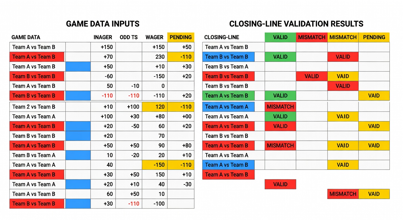
The practical test of a sports betting model is not calibration alone. It is closing line value (CLV). CLV measures whether the odds you receive at the time of bet placement are better than the odds the market closes at. If you bet a team at +120 (implied probability 45.5%) and the line closes at +105 (implied probability 48.8%), you have captured positive CLV. Over a large sample, positive average CLV predicts long-term profitability more reliably than win rate does.
Pinnacle's closing lines are the standard CLV benchmark. An operator like Bet365 or William Hill clips winning players through account restrictions; accordingly, their closing lines contain less pure market information. For CLV benchmarking purposes, Pinnacle's number is the reference.
Step 6: Bankroll Management
A Kelly staking system sizes bets as a fraction of the current bankroll proportional to the model's estimated edge. Full Kelly is theoretically optimal but produces high variance and requires exact edge estimates. Most practitioners use a fraction, typically between one-quarter and one-half Kelly, which reduces drawdown risk while preserving positive long-run expectation.
A half-Kelly stake on a bet where the model estimates a 3% edge over the closing line, with a bankroll of EUR 1,000, is approximately EUR 15 per bet. At that stake level, a 50-bet losing run reduces the bankroll by roughly 53%, which is recoverable. Full Kelly at the same edge would stake approximately EUR 30 per bet; the same losing run would reduce the bankroll by approximately 78%, which is not.
The model is only as good as its edge estimate. If the edge estimate is wrong, Kelly staking amplifies the error. Running the model in a paper-trading phase for a minimum of 200 bets before committing real money gives a sample sufficient to distinguish genuine edge from luck at a rough level of statistical confidence.